 The
linking number serves as another invariant in knot theory. Before
we delve into this, I need to define a few things. First of all,
according to Payne, the author of the website entitled "Knot Theory", a
link is a collection of knots, each which is a component of the link. [6]
See figure 18 for a picture of a link. Also, knots and links can
be assigned an orientation, which is a direction of travel around the knot
or link. It is obvious that there are only two possible orientations
for any knot or link. Another interesting fact concerning orientation
is that two knots which are equivalent without orientation are not in general
equivalent with orientation assigned to them.
The
linking number serves as another invariant in knot theory. Before
we delve into this, I need to define a few things. First of all,
according to Payne, the author of the website entitled "Knot Theory", a
link is a collection of knots, each which is a component of the link. [6]
See figure 18 for a picture of a link. Also, knots and links can
be assigned an orientation, which is a direction of travel around the knot
or link. It is obvious that there are only two possible orientations
for any knot or link. Another interesting fact concerning orientation
is that two knots which are equivalent without orientation are not in general
equivalent with orientation assigned to them.
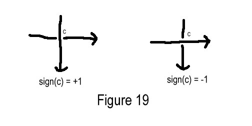
With these new facts in mind, we can describe the linking number invariant. Borrowing Murasugis definition, given an oriented link and a particular crossing point c in the link, we assign either +1 or -1 to c, and we write sign(c) = +1 or sign(c) = -1, according to whether the crossing is an overcross or an undercross. Of course, the definition of an overcross and an undercross must be consistent throughout the link. (see figure 19) Now say that we have a link L with two components K1 and K2. We can label all the crossing points between K1 and K2 with c1, c2, ..., cn. Finally we can define the linking number as lk(K1, K2) = 1/2{sign(c1) + sign(c2) + ... + sign(cm)}. [4]
Unfortunately, although the linking number is an interesting idea, it proves to be very difficult to calculate, and consequently is not a very useful invariant in determining equivalence of knots.
However, we will examine the proof that I
found in Murasugi's book showing that the linking number lk(K1, K2) is
an invariant of L. He tackles this proof by demonstrating that for
any link L with linking number n, when the Reidemeister moves are applied
to L until it is some equivalent link L`, L` will have linking number n
also. That is, the linking number is preserved under Reidemeister
moves.Reidemeister move #1 does not affect crossings between links, so
it is inapplicable, and therefore does not affect the linking number.
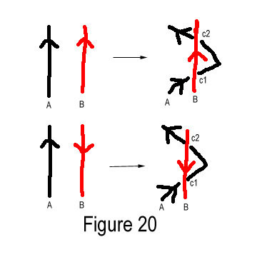
Reidemeister move #2 applies to two different cases according to the relative
orientations of the two knots which cross. Figure 20 shows that since
the new crossing points c1 and c2 created by the Reidemeister move have
different signs, the linking number will simply be sign(c1) + sign(c2)
= 0. Now we know that Reidemeister move #2 does not affect the linking
number.
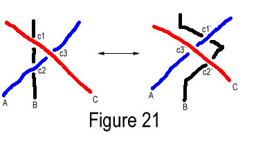 Consider
Reidemeister move #3. Let the three crossing points affected by the
move be called c1, c2, and c3, and their respective crossing points in
L` be called c1`, c2`, and c3`. Figure 21 demonstrates that sign(c1)
= sign(c2`), sign(c2) = sign(c1`), and sign(c3) = sign(c3`), regardless
of the orientations on strands A, B, and C of L. Now we have several
cases to consider. First of all, if A, B, and C belong to the same
component of L, then clearly we have an unaffected linking number.
Consider, however, the slightly more complicated case of where strand A
is of a different component than B and C. It is easily seen that
the only parts that have an effect on the linking number are sign(c2) +
sign(c3) and sign(c1`) + sign(c3`). However, recall that sign(c2)
= sign(c1`) and sign(c3) = sign(c3`). Therefore, these sums are equal
and accordingly ineffective on the linking number. Similar arguments
show that other combinations of the strands A, B, and C belonging to different
components of L results in no change in the linking number of L.
This suffices to prove that the linking number is really an invariant.[4]
Consider
Reidemeister move #3. Let the three crossing points affected by the
move be called c1, c2, and c3, and their respective crossing points in
L` be called c1`, c2`, and c3`. Figure 21 demonstrates that sign(c1)
= sign(c2`), sign(c2) = sign(c1`), and sign(c3) = sign(c3`), regardless
of the orientations on strands A, B, and C of L. Now we have several
cases to consider. First of all, if A, B, and C belong to the same
component of L, then clearly we have an unaffected linking number.
Consider, however, the slightly more complicated case of where strand A
is of a different component than B and C. It is easily seen that
the only parts that have an effect on the linking number are sign(c2) +
sign(c3) and sign(c1`) + sign(c3`). However, recall that sign(c2)
= sign(c1`) and sign(c3) = sign(c3`). Therefore, these sums are equal
and accordingly ineffective on the linking number. Similar arguments
show that other combinations of the strands A, B, and C belonging to different
components of L results in no change in the linking number of L.
This suffices to prove that the linking number is really an invariant.[4]
